R is very powerful but awful to teach students to use. My students almost universally detest it because they have to learn to code. Unfortunately they haven’t much option but to use it to get stats done! (XLSTAT anyone?) So I wanted to throw out a quick post detailing how to carry out an ANOVA in R and interpret the output the easy way. Most importantly I don’t want to get into the mechanics of R or the theory of stats. I’m far from an expert in either but this is the simplest and most common test I need to get students to perform so hopefully this will save them and me a lot of headaches in future.

First you need a data set saved in comma separated value format (.csv) with a header row containing the name of each variable. Open a spreadsheet and copy your data into this format with one row of variable names at the top of the sheet and numbers in the column below. You may only have one header row and you can’t use spaces in the names. If you must use multiple words for variable names separate them with underscores.

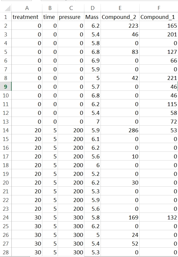
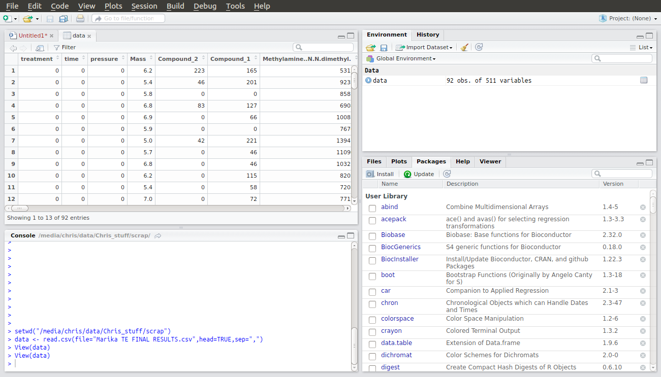
In this example each row contains data for one sample. The first four columns characterise the experimental treatments the samples have been subjected too and the mass of sample analysed. You don’t need sample names or numbers, although it doesn’t matter if they are in there. They’re just not necessary for your stats. What the rest of the columns in this data set are doesn’t matter. As it happens they are peak areas from the GC-MS but they could be cell counts or enzyme activity or whatever you’re measuring. You should arrange your data like this in Excel and save the sheet as a .csv file in a convenient folder that you can label something like “stats” or “results”.

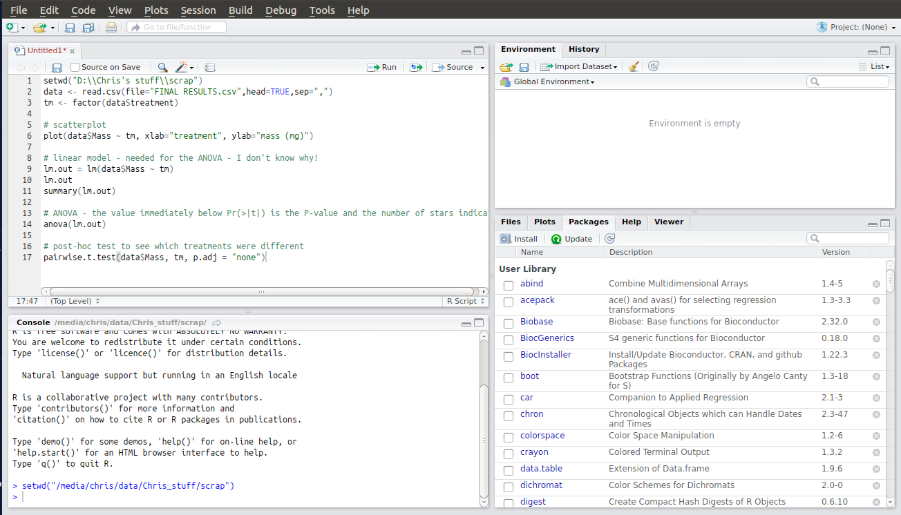
Next, open R Studio and create a new script file by pressing Ctrl + Shift + N. Then press Ctrl + S and save it in the same folder as your .csv file with an appropriate name. Then copy this text into it and save it in the same folder as your .csv file:

setwd(“D:\\Chris’s stuff\\scrap”)
data <- read.csv(file=”FINAL RESULTS.csv”,head=TRUE,sep=”,”)
tm <- factor(data$treatment)

# scatterplot
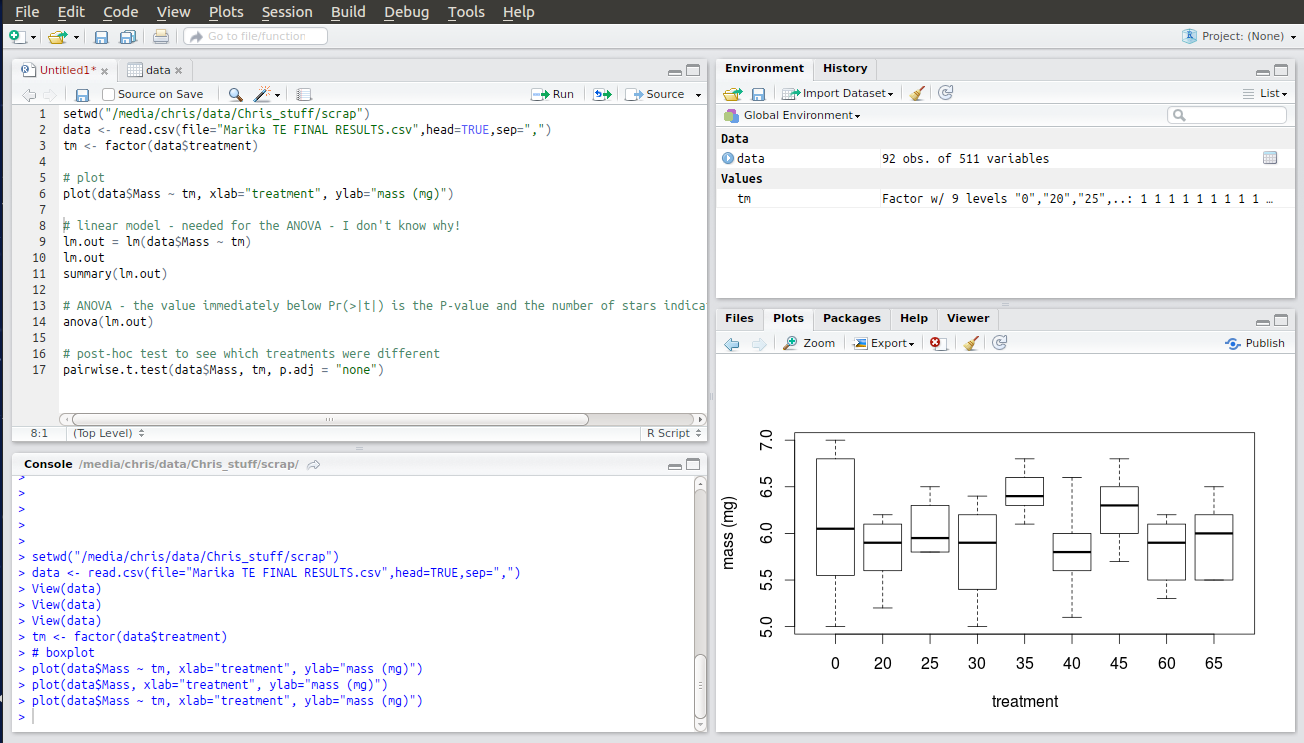
plot(data$Mass ~ tm, xlab=”treatment”, ylab=”mass (mg)”)

# linear model – needed for the ANOVA – we don’t care why!
lm.out = lm(data$Mass ~ tm)
lm.out
summary(lm.out)

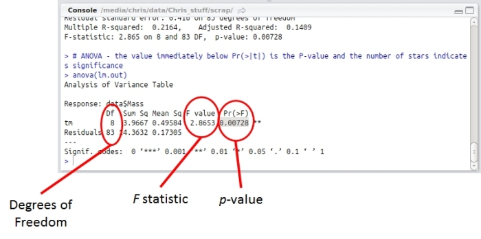
# ANOVA – the value immediately below Pr(>F) is the p-value and the number of stars indicates significance
anova(lm.out)

# post-hoc test to see which treatments were different
pairwise.t.test(data$Mass, tm, p.adj = “none”)

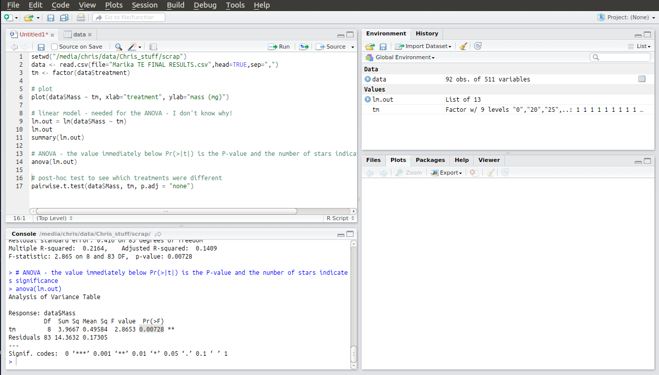
You will need to edit some of the text to reflect your own computer’s file paths. The first line, for example, is just an example and points to the scrap directory on my laptop. You will need to correct this to point to the directory you have created with your .csv file in. To do this press Ctrl + Shift + H, navigate to the folder and click “OK”. This won’t change the script but instead the new relevant piece of code will appear in the console output. Copy and paste this into your script to replace my version. Here’s what it looks like when I do this and select a scrap folder on my other PC:

Note that this isn’t as simple as copying and pasting a folder path in Windows! R requires that the forward slashes in the file path be escaped, or doubled up, so that it doesn’t mistake them as some sort of function. Google it if you want to know more.

Next, you need to replace the name of my .csv file with yours. Make sure you don’t delete the speech marks. You now have two lines of code which will allow you to load your csv file into R. When you run these lines an entry will appear under Data in the Global Environment window. If you double click on it you will see a table of your data open in the Files window.

In this data set the first column contains numbers that are not data but that are a code for the various treatments in this experiment. We don’t want R to treat these numbers as numbers, but as categories. Therefore the third line of code in the script tells R to create something called a factor to use as categories to interpret your data but not to use as numerical values. When you run this line you will see another entry in the Global Environment window confirming that R has created a new factor called “tm” with the numbers as names for each treatment category.

The next line of code allows you to plot your data by category. A useful way of viewing the distribution of your data before you start looking for statistical differences. The two things to plot are specified as “data$Mass ~ tm“. This tells R to take the continuous numerical data in the column titled Mass (N.B. – case sensitive!) from the dataset called “data” and plot it against the factor called “tm“. R will create a boxplot of the numerical data for data$Mass showing the distribution of the data. You should be able to guess, at this stage, whether you are going to get a significant result. I’m pretty sure that treatment 35 is going to be significantly different from treatment 40!

The next few lines of code construct something called a linear model. I’m honestly not sure why R needs this to do the ANOVA. Like I said, I’m not an expert but it won’t work without them so you better go ahead and run them! The output is a table that you don’t need to interpret. Ignore it.

The second to last line is the code to run the actual ANOVA. Running this produces an ANOVA table with the results of your analysis as a p-value under Pr(>F). If p < 0.05 one or more of your treatments is significantly different from the rest. I’ve highlighted my result here.

R is kind enough to annotate your result with stars indicating just how significant it is. My p-value was less than 0.01 so it got two stars. Whoop!

The final piece of code is something called a post-hoc test to determine which treatments are statistically different from each other. This is important as ANOVA doesn’t tell you this. It just tells you that something is different and not what. The pairwise t-test does tell you what and presents a t-statistic for each pair to let you know just how different. Interestingly the first column of results are the same as the output of the linear model. In the pairwise table they’re more easily interpreted and there’s results for all the other pairwise comparisons too, so much more informative.

Importantly, if the ANOVA result is not significant you must accept the null hypothesis, even if the pairwise tests appear to show a statistically significant result. Its not an either/or scenario. ANOVA is more sensitive than t-test and is the determinative component. If the ANOVA is not significant the t-test results are meaningless, whatever their values!

Edit 13-04-2017: The last thing to mention, which really should have been the first, is this: if your data does not comply with the assumptions of ANOVA you cannot use this test anyway. Data for ANOVA must be independent and exhibit homogeneity of variance (heteroscedacity). There is a common misconception that data for ANOVA must be normally distributed too. Tony Underwood has shown that ANOVA is relatively robust to non-normal data sets.