Making Size Exclusion Chromatography columns

My summer student, Kalita, has been digesting oligosaccharides, derivatising them and injecting them into the mass spectrometers in an effort to derive structural information from these complex molecules. We had hoped to use acrylamide gel electrophoresis to visualise the performance of our digests, in the way of Pomin et al (2005).

Screenshot from 2016-03-03 20:30:41.png

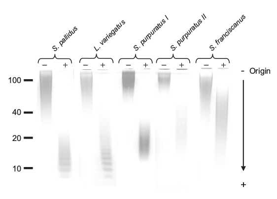
This figure from the paper shows the effect of their hydrolysis technique upon the molecular weight of the oligomer. Note the banding patterns resulting from selective hydrolysis of certain glycosidic bonds. This produces a regular reduction in size of the fragments. We wanted to use this feature to produce polymeric fragments in the <10kDa size rage. These would be amenable to LC-MS/MS, as in Lang et al (2014), allowing us to infer the sequence, functionalisation and bonding of the monomers within the oligomer.

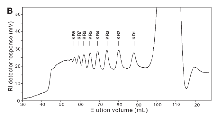
As it turned out our acrylamide gels got lost somewhere amidst The Great Bureaucracy and so, with time running out we cast around for alternate technologies. Enter Yang, et al (2009), who used a similar technique in their paper, but also deployed Size Exclusion Chromatography to illustrate the size-class of fragments produced.

Screenshot from 2016-03-03 21:11:31.png

The thing is we didn’t have any GPC or SEC columns.  😦


So we decided to try making our own!  😀


Fortunately or chemical store had a shelf of old bottles of dextran and other GPC or ion-exchange substrates. We dug up a protocol from an MSc thesis by Wilfred Mak in which he’d used an anion exchange substrate to determine the molecular weight of intact sulfated fucan oligosaccharides, rifled through the stores to find some substrates that looked about right and away we went!

We started out with a biuret:

IMG_20160302_172848.jpg

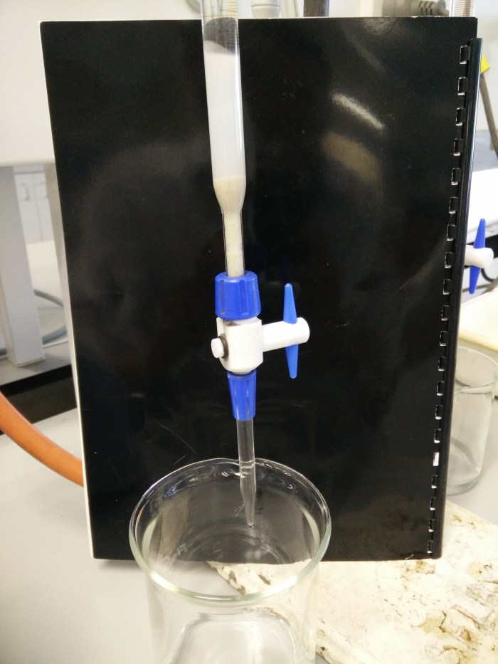
At the bottom, hidden by the blue compression screw, is a plug of deactivated glass wool with a few mL of sand on top of that and then the white dextran gel. This was the first addition of substrate and settling. After topping it up we have a column of about 40cm length. This type of column is purely gravity-fed. You add sample and running buffer at the top and wait for the head of fluid to pass through the column, collecting fractions through the tap at the bottom. This can take hours.

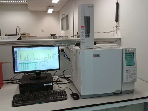
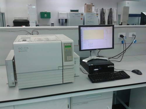
While Kalita was putting this together I was looking at some of the old silica particle LC columns I had and wondering if I might dismantle them, remove the packing and repack them with the dextran to give a real, high-pressure column. This could be plumbed into one of our conventional LC setups, allowing us to push samples through at a faster rate and giving the option of automated sample injection, data and fraction collection. I had something of a brain wave and realised that I had some Swagelok fittings which would allow me to fit a piece of 1/4″ polypropylene air line with pressure-tight caps and LC fittings at either end to fulfil exactly that function. A couple of hours later Kalita and I were the proud parents of monstrous creation on the left!

IMG_20160303_162725.jpg

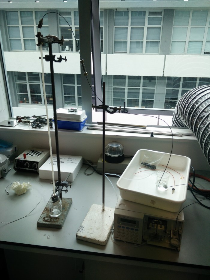
The white tube held between the two clamps on the left hand retort is the air line packed with hydrated dextran. The line at the top comes from the Shimadzu LC pump on the right, which is pumping Tris buffer through the column to settle the packing material. We can get a flow of 2 mL/min through the column with a back pressure of about 5 bar. Plenty for LC!

For now our creation is parked until we can get round to doing something cool with it on Monday but watch this space to see the outcome. Our intention is to add an autosampler to the front for sample injection, a Refractive Index Detector and maybe even an electrochemical detector on the outflow to detect what came off the column and possibly even a fraction collector for downstream LC-MS/MS analysis of the fractions! Fun!

Our first goal is to validate the SEC function by injecting a range of proteins stained with Bradford Reagent. We can also try some di- and tri-saccharides along with our oligo digests.


References cited

Lang et al (2014). Applications of Mass Spectrometry to Structural Analysis of
Marine Oligosaccharides. Mar. Drugs 2014, 12, 4005-4030
doi:10.3390/md12074005

Pomin et al (2005). Mild acid hydrolysis of sulfated fucans: a selective 2-desulfation reaction and an alternative approach for preparing tailored sulfated oligosaccharides. Glycobiology vol. 15 no. 12 pp. 1376–1385, 2005
doi:10.1093/glycob/cwj030

Yang et al (2009). Mechanism of mild acid hydrolysis of galactan polysaccharides with highly ordered disaccharide repeats leading to a complete series of exclusively odd-numbered oligosaccharides. FEBS Journal 276 (2009) 2125–2137
doi:10.1111/j.1742-4658.2009.06947.x

Advertisement

liquid chromatography of photosynthetic pigments

I’m developing a method for quantifying photosynthetic pigments with liquid chromatography. I started out just mashing up a couple of leaves from some plants in the teaching lab. A begonia leaf and a tobacco leaf. Here’s the begonia leaf before grinding:

begonia leaf pigment extraction 2

And after grinding in acetone:

begonia leaf pigment extraction

I centrifuged the liquid to remove particulates and diluted some of the supernatant in a little more acetone as that bright green colour was probably too concentrated to inject directly.

I initially tried using the diode array detector and the mass spectrometer in tandem so that I could confirm identities of DAD peaks with the mass spectrum but I think the sensitivity of the mass spec was too low. The pigments absorb light pretty strongly, as you might expect, so you don’t need to inject high concentrations to get a signal from an absorbance detector. So I gave up using the mass spec and just looked for peaks in the DAD. Initially I just infused them straight through the DAD without using an LC column so that I could confirm that I could see peaks at the right wavelengths. Plant pigments fall into several different categories. I was expecting to see chlorophylls, which are common to all plants, as well as some xanthophylls and/or carotenoids. We happened to have some carotene in our chemical store so I prepared a standard dissolved in acetone to inject as a reference.

The direct injections worked well with large peaks visible at 440nm (xanthophylls/carotenoids) and 640nm wavelengths (chlorophyll). The carotene showed up very nicely at 440nm, as expected, with nothing visible at 640nm. Next I wanted to see how many different pigments I could separate but I wanted to do it really quickly, without setting up a full LC gradient. So I ended up trying just a Phenomenex C8 guard column in a holder instead of an actual analytical LC column and set a 1 minute gradient from 20 to 100% isopropanol. I had to use isopropanol, instead of the more usual acetonitrile or methanol, because these pigments are quite hydrophobic. This seemed to work well so I stretched the gradient out to 6 minutes and ran them again (yes, I ended up running a full gradient after all but it was worth building up to it). As you can see from my quick-and-dirty method it actually worked beautifully:

pigments HPLC C8 guard column

This rather busy chromatogram shows several different plots. The two relevant ones are the pink one (440nm) and the black one just above it (640nm). The peaks in these plots represent different pigments in their respective classes. There’s five xanthophylls or carotenoids and at least three chlorophyll peaks (the last one is two peaks coeluting). The last of the pink peaks happens to coelute perfectly with my carotene standard and they shared the same absorbance spectra. Each pigment tends to have a unique absorbance spectra corresponding to its role in absorbing different wavelengths of light. The plot below shows the five xanthophyll/carotenoid peaks and their respective absorbance spectra.

pigments HPLC C8 guard column - xantho & caro peak spectra

All in all a pretty successful day’s HPLC! I’m looking forward to applying this to some marine benthic sediments tomorrow to see what sort of pigments are present in the microphytobenthos. I’m also now well set up to investigate the pigments in the giant springtails I mentioned recently.

A useful paper for background and huge amounts of detail about pigment HPLC is Bidigaire et al, (2005):

Bidigare, R. R., L. Van Heukelem and C. C. Trees. 2005. Analysis of algal pigments by high-performance liquid chromatography. In: Algal Culturing Techniques (R. A. Andersen, Ed.), Academic Press, New York, pp. 327-345.

Shimadzu gas chromatographs

This is the Shimadzu GC-2010 Plus, our newest gas chromatograph:

image

 The tower mounted on top is the AOC-20i autoinjector. We also have another two GC-210s with autoinjectors and a pair of venerable GC-17As.

image

These instruments are used for quantitative analysis of small biomolecules such as fatty acids, amino acids and sugars in organisms, biofluids and food products as well as for profiling the volatile compounds associated with food flavours by Solid Phase Micro Extraction [SPME]. 

We have a wide range of columns to choose from but two phases that seem to separate most analytes are 5% phenyl, such as Zebron ZB-5, for less polar compounds and wax columns, such as the Zebron DB-WAX, for more polar things. The GC-2010 Plus is fitted with a Restek FAMEWAX column for Fatty Acid Methyl Ester [FAME] analysis and is routinely used to separate and quantify 36 different FAMEs.

Fatty acids are not volatile in the GC and so cannot be analysed natively. A while ago though, some clever chaps realised that you could esterify fatty acids to make them volatile. This is hugely advantageous as fatty acids are not especially amenable to liquid chromatography either. This method has been refined over the years and we now use a one-tube esterification and extraction method based on de La Cruz Garcia et al (2000). The plots below show a chromatogram of a Supelco FAME standard and below that the FAMEs from a sample of human plasma. Tridecanoic acid is the internal standard.

Another application of our GCs is to analyse sugars. Sugars are even harder to analyse than fatty acids because they are so polar, they do not absorb light strongly and they are not volatile. We use the method of Blakeney et al (1983) to convert sugars from non-volatile compounds to volatile alditol acetates amenable to GC analysis. Here is a chromatogram from our GC-MS showing peaks for ten alditol acetylates in a standard mixture:

image

sugar and retention time (mins)

  • erythritol  6.43
  • rhamnose  9.93
  • fucose  10.17
  • xylose  10.62
  • allose  16.40
  • inositol  16.57
  • glucose  17.83
  • galactose  18.06
  • mannose  18.70

References 

Blakeney A.B., Harris P.J., Henry R.J., Stone B.A. (1983). A simple and rapid preparation of alditol acetates for monosaccharide analysis. Carbohydrate Research 113:2 p291–299

de La Cruz Garcia, Lopez Hernandez, Simal Lozano (2000). Gas chromatographic determination of the fatty-acid content of heat-treated green beans. Journal of Chromatography A. 891:2 p367–370

stability of neonicotinoid LC-MS standards
I’ve got mixed standards of six neonicotinoid pesticides for my LC-MS analysis that have been sat in the autosampler for more than six months. I’m getting ready to do some more so I thought it was time to make up a new mixed working solution and standard curve. Blow me if the response of the new standard didn’t match the old one almost perfectly! 

This is remarkable because it shows that neonicotinoids are perfectly stable in 5% acetonitrile at 6 degrees C and in brown autosampler vials.