
Proud to have voted for the NZ Green Party tonight. Looking forward to seeing a change of government and some investment in good scientific research and sustainable technological development as well as protection of our beautiful land, sea and sky.
Author: drchrispook

stability of neonicotinoid LC-MS standards
I’ve got mixed standards of six neonicotinoid pesticides for my LC-MS analysis that have been sat in the autosampler for more than six months. I’m getting ready to do some more so I thought it was time to make up a new mixed working solution and standard curve. Blow me if the response of the new standard didn’t match the old one almost perfectly!
This is remarkable because it shows that neonicotinoids are perfectly stable in 5% acetonitrile at 6 degrees C and in brown autosampler vials.
Auckland Winter humidity problems
I’ve got a climate datalogger in my house here in West Auckland. Its based on an Etherten from Freetronics, which is an ethernet-enabled Arduino Uno compatible board. On that is sat a wing screw shield for easy connection of wires and on top of that is sat an Adafruit LCD shield showing the readings.
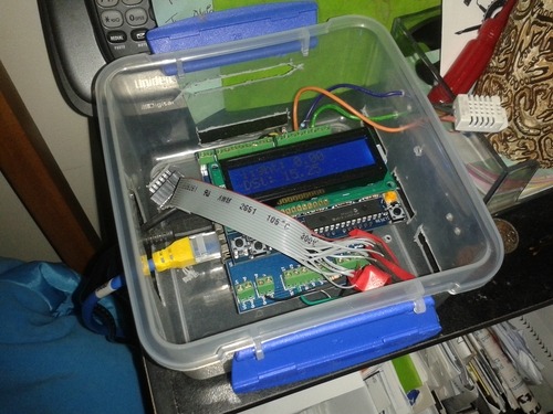
Inside or outside it are a DHT22 temperature and relative humidity sensor, a BMP085 air pressure and temperature sensor, a DS18B20 temperature sensor and a light dependent resistor. The sensors are polled every 20s and the data uploaded to Xively. The BMP temperature sensor reads a few degrees high because its inside the plastic box, exposed to the warmth from the circuitry. The DS18B20 generally reads a couple of degrees low because its hanging down the back of the shelves the logger sits on, away from ambient air movement (although this is, of course, still interesting [to me, anyway]). The whole affair runs off a 5V power supply connected by USB.
Here’s a shot of the log from the last few days. The gap in the data is where the logger hung and had to be reset, by the way.

As you can see, after a series of cold, wet days- indicated by the small peaks in the ‘light’ plot at the top left- relative humidity climbs to nearly 100%. This is despite us leaving the heat pump and a pair of heaters running all night. This was not helped at all by the need to dry clothes inside when its too wet outside, adding to the moisture in the air.
As a consequence I now have mould growing on the shelves in my bedroom!

Yay, for houses with poorly fitting, single-glazed windows and no insulation!
Here’s the Arduino sketch, if anyone’s interest.
#include <SPI.h>
#include <Ethernet.h>
#include <HttpClient.h>
#include <Cosm.h>// ! ! USB DEBUG OPTION ! !
int debug = 0;// Sensor setup
#include “Wire.h”
#include “Adafruit_BMP085.h”
#include “DHT.h”
#include <OneWire.h>
#include <DallasTemperature.h>
#include <Adafruit_MCP23017.h>
#include <Adafruit_RGBLCDShield.h>// MAC address for your Ethernet shield
byte mac[] = { 0xDE, 0xAD, 0xBE, 0xEF, 0xFE, 0xED };
IPAddress ip (192,168,1,65); // Available Static IP address on your Network. See Instructions// Your Cosm key to let you upload data
char cosmKey[] = “@@@@@ your key goes between the quotes here @@@@@@@”;#define FEED_ID 76854;
unsigned long feedID = FEED_ID;// Define the strings for our datastream IDs
char sensorID0[] = “BMPp”;
char sensorID1[] = “DHTh”;
char sensorID2[] = “DSt”;
char sensorID3[] = “light”;
char sensorID4[] = “BMPt”;
char sensorID5[] = “DHTt”;CosmDatastream datastreams[] = {
CosmDatastream(sensorID0, strlen(sensorID0), DATASTREAM_FLOAT),
CosmDatastream(sensorID1, strlen(sensorID1), DATASTREAM_FLOAT),
CosmDatastream(sensorID2, strlen(sensorID2), DATASTREAM_FLOAT),
CosmDatastream(sensorID3, strlen(sensorID3), DATASTREAM_FLOAT),
CosmDatastream(sensorID4, strlen(sensorID4), DATASTREAM_FLOAT),
CosmDatastream(sensorID5, strlen(sensorID5), DATASTREAM_FLOAT),};
// Finally, wrap the datastreams into a feed
CosmFeed feed(feedID, datastreams, 6 /* number of datastreams */);EthernetClient client;
CosmClient cosmclient(client);// LCD shield
Adafruit_RGBLCDShield lcd = Adafruit_RGBLCDShield();
#define WHITE 0x7Adafruit_BMP085 bmp;
//
//// Data wire is plugged into which pin on the Arduino?
#define ONE_WIRE_BUS 6
//
//// Setup a oneWire instance to communicate with any OneWire devices (not just Maxim/Dallas temperature ICs)
OneWire oneWire(ONE_WIRE_BUS);
//
//// Pass our oneWire reference to Dallas Temperature.
DallasTemperature sensors(&oneWire);#define DHTPIN 3 // what pin we’re connected to
#define DHTTYPE DHT22 // DHT 22 (AM2302)
DHT dht(DHTPIN, DHTTYPE);float light;
void setup() {
// put your setup code here, to run once:
Serial.begin(9600);
lcd.begin(16, 2);
lcd.setBacklight(WHITE);
lcd.print(“initialising”);Serial.println(“Starting single datastream upload to Cosm…”);
Serial.println();if (debug < 1 ) {
while (Ethernet.begin(mac) != 1)
{
Serial.println(“Error getting IP address via DHCP, trying again…”);
Serial.println(millis());
// lcd.clear();
lcd.setCursor(0,0);
lcd.print(“Error getting IP”);
lcd.setCursor(0,1);
lcd.print(millis()/1000);
delay(5000);
}
}// set pin modes to power sensors
pinMode(7, OUTPUT);
pinMode(5, OUTPUT);
pinMode(4, OUTPUT);
pinMode(2, OUTPUT);digitalWrite(7, LOW);
digitalWrite(5, HIGH);
digitalWrite(4, LOW);
digitalWrite(2, HIGH);// initialise sensors
bmp.begin();
dht.begin();
sensors.begin();delay(100);
}
void loop() {
lcd.clear();
lcd.setCursor(0, 0);
lcd.print(millis()/1000);// Get sensor readings
// BMP085
float BMPt = bmp.readTemperature();
float BMPp = bmp.readPressure() / 100.0;// DHT22
float DHTh = dht.readHumidity();
float DHTt = dht.readTemperature();// DS18B20
sensors.requestTemperatures(); // Send the command to get temperatures
float DSt = (sensors.getTempCByIndex(0));// get light
light = analogRead(0)/ 10.23;datastreams[0].setFloat(BMPp);
datastreams[1].setFloat(DHTh);
datastreams[2].setFloat(DSt);
datastreams[3].setFloat(light);
datastreams[4].setFloat(BMPt);
datastreams[5].setFloat(DHTt);if (debug > 0) {
/*———–( Show the values inside the streams for test/debug )—–*/
Serial.println(“—–[ Test: Check values inside the Streams ]—–”);
Serial.print(“BMPp: ”);
Serial.println(datastreams[0].getFloat()); // Print datastream to serial monitor
Serial.print(“DHTh: ”);
Serial.println(datastreams[1].getFloat()); // Print datastream to serial monitor
Serial.print(“DSt: ”);
Serial.println(datastreams[2].getFloat()); // Print datastream to serial monitor
Serial.print(“light: ”);
Serial.println(datastreams[3].getFloat()); // Print datastream to serial monitor
Serial.print(“BMPt: ”);
Serial.println(datastreams[4].getFloat()); // Print datastream to serial monitor
Serial.print(“DHTt: ”);
Serial.println(datastreams[5].getFloat()); // Print datastream to serial monitor
delay(2500);
}if (debug < 1) {
Serial.println(“Uploading to Cosm”);
lcd.clear();
lcd.setCursor(0,1);
lcd.print(“sending to COSM”);
int ret = cosmclient.put(feed, cosmKey);Serial.print(“COSM client returns: ”); // Get return result code, similar to HTTP code
lcd.clear();
lcd.setCursor(0,0);
lcd.print(“COSM client”);
lcd.setCursor(0,1);
lcd.print(“returned: ”);
Serial.println(ret);
lcd.print(ret);
Serial.println();
delay(500);
lcd.clear();
lcd.setCursor(0,0);
lcd.print(“BMPp: ”);
lcd.print(BMPp);
lcd.setCursor(0,1);
lcd.print(“BMPt: ”);
lcd.print(BMPt);
delay(3500);
lcd.clear();
lcd.setCursor(0,0);
lcd.print(“DHTh: ”);
lcd.print(DHTh);
lcd.setCursor(0,1);
lcd.print(“DHTt: ”);
lcd.print(DHTt);
delay(3500);
lcd.clear();
lcd.setCursor(0,0);
lcd.print(“light: ”);
lcd.print(light);
lcd.setCursor(0,1);
lcd.print(“DSt: ”);
lcd.print(DSt);
delay(3500);
}
}
I love HPLC – High Pressure Liquid Chromatography
HPLC is my favourite analytical technique because it can be applied to pretty much anything soluble. Which includes, well, pretty much everything. This is in contrast to Gas Chromatography (GC), which only works for compounds which are volatile at temperature below about 350C. This is only about 5% of molecules so that’s a fairly restrictive condition, although as us scientific types are jolly clever we’ve worked out cunning ways of changing non-volatile molecules we want to analyse by GC to make them volatile.
Here’s a link to one of the HPLC systems we use in our labs, including some of the applications for this technique. In addition I’d like to present a bit of my history with this technique to provide some examples of what it can achieve.
I used HPLC during my PhD to quantify glutathione ratios in the polychaete worm I was studying. Glutahione ratios are a very useful indicator of oxidative stress as glutathione is the first line of defence against the toxic effects of many metals and is a substrate or cofactor in many antioxidant and other enzymes.
Whilst working on my PhD I also used HPLC to quantify hormones in monkey pooh! This was a quick bit of work to validate a friend’s work looking at social hierarchies in communities of monkeys in zoos. The hormones in their pooh were correlated with their health and with their place in the hierarchy!
Nowadays you tend to find HPLC systems coupled to Mass Spectrometers, harnessing the resolving power of this technology to enhance the capabilities of liquid chromatography. This allows you to identify and quantify many different compounds in very short runs and in very complex matrices such as urine, blood and cell or tissue homogenates. SoAs was lucky enough to acquire an Agilent 6420 triple quadrupole mass spectrometer and an Agilent 1200 series LC stack a couple of years ago and this has become the workhorse of our lab.
During my PhD I first managed to get time on an LC-MS instrument when I was based at Plymouth University, where I worked as Research Assistant on a project characterising the metabolism of a common biocide, 2-hydroxybiphenyl [HBP], in common shore crabs. This was incredibly valuable experience and I was lucky to have an oustanding LC-MS mentor in the form of Dr Claire Redshaw. Claire helped me develop a method to extract HBP and its metabolites from urine we collected from the crabs (that’s a post for another day). The LC-MS allowed us to confirm that the metabolites were mostly sulphate-conjugates of either the parent molecule or of a monooxygenated product of Phase 1 detoxification.
Other pieces of LC-MS work I’ve been involved in or conducted myself include the extraction and quantification of bisphenol A from human urine, profiling of triglycerides in edible oils and in human plasma and the quantification of neonicotinoid pesticides in pollen and honey. I have been working on the latter piece of work for several years now, starting with a postdoc position at Exeter University studying the toxicity of this class of pesticides to bees and continuing now here at AUT.
Hopefully these examples of HPLC and LC-MS applications illustrate why I love the technique so much. One reason which may not be obvious is that LC is a notoriously challenging technique and can be incredibly complex to get right. So much so that it is often referred to as a “Black Art”. I have a favourite joke I tell to all the students when their analysis isn’t working as it should: I ask them how big their chicken was that morning. When they look baffled or alarmed I follow up with the question: “Well, you did sacrifice a chicken this morning, didn’t you?”
LOL!
Shimadzu LC20 series HPLC
I’m going to start a page for each of my instruments detailing what it does and giving some details of what it gets used for. I’m going to start with our Shimadzu LC20 series High Pressure Liquid Chromatograph [HPLC]. HPLC is my favourite analytical technique and I have more than 10yrs experience getting results from it.
Here’s a picture of the beast:

The system is comprised of a quaternary LC pump with integrated degassing; high speed, flushed-path, total-volume sample injection, thermostatted autosampler for up to 70 samples; a venerable Jones Chromatography column heater (HOT!); a twin wavelength UV-visible absorbance detector and a fluorescence detector. The system is connected to a PC running LC Solution. The autosampler and degassing unit were both new this year, replacing functional but less capable units which have been transferred to a secondary system. We now have the ability to run two separate HPLC systems fully automatically.
Apart from our flagship LC-MS this is our most capable and modern LC system and has been responsible for almost all of the HPLC-based research output. Here’s a few of the compounds this system has been used to identify and quantify:
- the anticancer drug gemcitabine and its metabolites
- cafffeine & its metabolites in human plasma and urine
- sex steroids in scallop gonads
- monosaccharide profiles using phenyl methyl pyrazolone derivatisation
- methyl anthranilate in grapes
The cutting edge of HPLC technology has moved beyond systems like this one to Ultra-High Pressure Liquid Chromatography (UPLC). However, its great to have a sturdy and capable workhorse system like this one for the more straightforward bits of analysis.
AUT Marine Biologist calls for free plastic bags to be banned
Great work from Steph Borrelle of AUT’s Institute for Applied Ecology NZ.
David Colquhoun on ‘Should metrics be used to assess research performance?’
David is an astonishingly highly esteemed and energetic firebrand academic who writes a blog dedicated to scientific rigour, integrity and public dissemination. He’s just put up this post presenting a draft submission to the UK HEFCE on the use of metrics and other performance measures in the allocation of funding. You should read it.
DC is also on twitter: @david_colquhoun
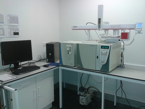
new Gerstel MPS
In a moment of stunning brilliance on my part I managed to convince the school to purchase an autosampler for our Thermo GC-MS. This wasn’t actually that difficult once I’d pointed out that the $120,000 instrument was effectively unusable for research without one.
After a lot of contemplation we opted for the Gerstel Multi-Purpose Sampler as this seemed to be the most flexible platform and wasn’t manufacturer-specific. This was an important consideration given the 10 year age of the GC-MS so if we upgraded to an Agilent GC-MS in the next few years <cough! cough! Hint, hint> then we’d be able to transfer it to the new instrument without issue.
The MPS was installed about 6 weeks ago and has already injected more samples into the GC-MS than it saw in most of the previous year! Awesome is the power of automation! I cannot wait to set up some automated sample prep. I am really keen to try methyl chloroformate derivatisation for metabolite profiling of biogenic amines, organic acids and other small metabolites. Silas Villas-Boas of Auckland University School of Biological Sciences and his PhD student Sergey Tumanov very kindly shared their method (1) and library with me and I have been itching to try it out.
Many thanks to Gerstel for a beautifully constructed and controlled instrument and also to Udo Rupprecht of Lasersan for doing the install and providing support.
Here’s a picture of the beast. You can almost smell the barely contained analytical potential!
;-D
Reference
(1) Smart, K. F.; Aggio, R. M. B.; VanHoutte, J. R. and Villas-Bôas, S.G. 2010. Analytical platform for metabolome analysis of microbial cells using methyl chloroformate derivatization followed by gas chromatography-mass spectrometry (GC-MS). Nature Protocols 5: 1709 – 1729. doi:10.1038/nprot.2010.108
logging thermocycler performance
My favourite PhD student (hi, squids!) was having issues with her PCR. She was ending up with empty tubes at the end of her program and was concerned that the machine wasn’t producing the right temperature cycle. As I had an Adafruit MAX6675 thermocouple board on my desk I offered to log the cycle to determine whether this was the case. I used a miniature breadboard to connect the Arduino Nano and MAX6675 breakout. The measurements were output to serial and logged to text file by a PC running my Processing datalogger sketch. Here’s the result:
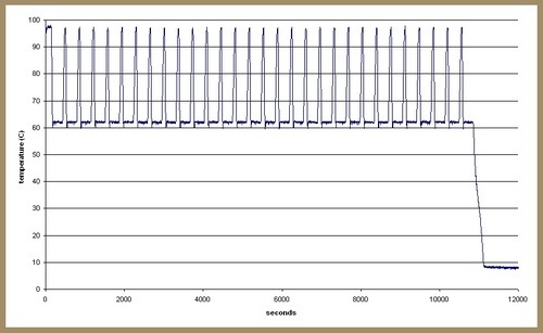
There seems to be some real issues here as the temperatures don’t match the program well at all. There’s meant to be a 55C step immediately before each polymerisation hold at 62C and the sensor gets no where near this. This might be a result of poor heat transfer between the reaction tubes and the thermocouple but I figure that accurately reflects the same process of heat transfer between the block and the liquid in the reaction tubes.
I’ve run the test again in a different well on the block. I’ll need to validate the thermocouple’s temperatures using another couple of thermometers to make sure its giving accurate temps but just this initial test has revealed a problem worthy of serious investigation. The fun continues another day … .
blog reboot
I am in the process of rebooting this thin initial attempt at blogging. Hopefully I will be able to turn out a couple of posts a week detailing what I get up to in the lab and sharing some of the toys I get to play with.
